
Require user to enable macros
This module demonstrates:
- Construction of a Macro Warning worksheet that requires the user to enable macros
- The code to handle the Enable Content event of the macro Warning worksheet
- The code to reset the Macro Warning worksheet before distribution to the user
1. Macros disabled security warning
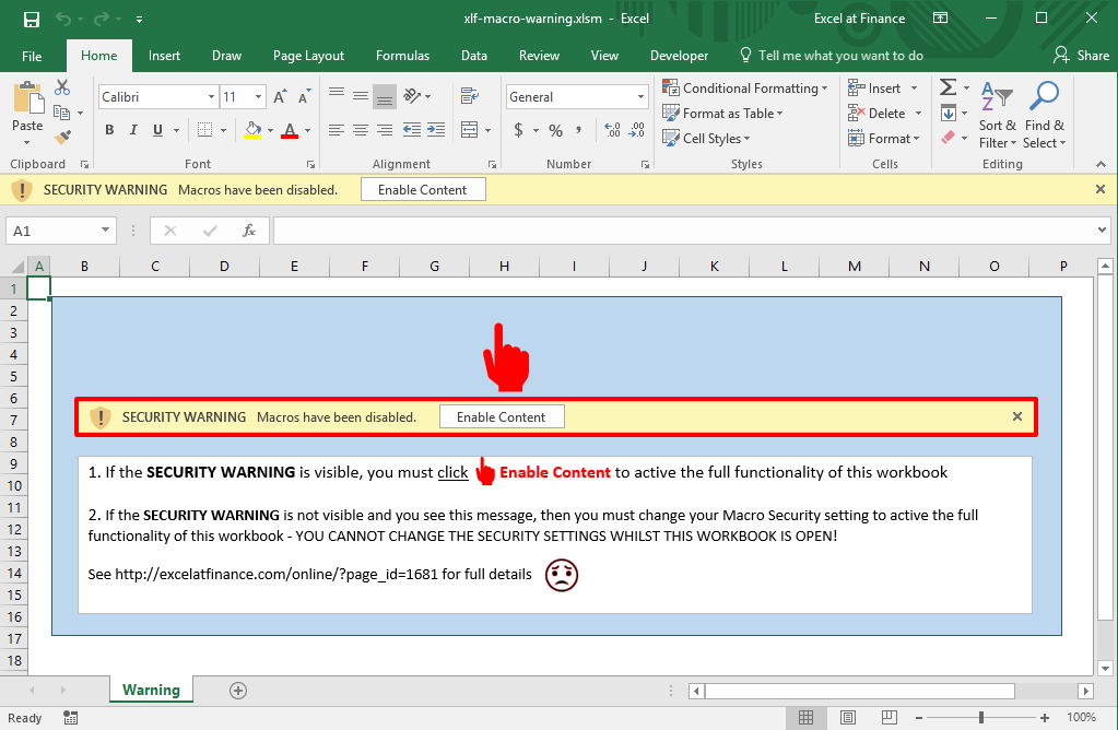
Inexperienced spreadsheet users often overlook the Enable Content security warning displayed when an xlsm file is opened. They become perplexed when UDFs display a #NAME? error or macros do not appear on the Macro list. A useful solution is to hide the contents of the workbook until macros are enabled. When the workbook is opened, and if macros are not enabled, then the user is presented with the Warning Message as shown in figure 1. The process involved, message construction, activation, and resetting is shown in the following sections.
Elements of the warning worksheet
Here are the details of selected items from the worksheet in figure 1:
- The worksheet (stage 1)
- Gridlines: hidden by code (code 2
ResetWarning, line 19) - Column A width (Height: 2.14 (20 pixels) set to same dimension as height (Height: 15.00 (20 pixels)), merely for presentation purposes
- Gridlines: hidden by code (code 2
- The blue background
- Name (displayed in the name box): Rectangle 1
- Drawing Tools contextual tab
- Created by: Insert > Illustrations > Shapes > Rectangle
- Size: Format > Size Shape Height: 8.2 cm, Shape Width: 24.45 cm
- Fill: Format > Shape Styles > Shape Fill > Theme Colors Blue, Accent 5, Lighter 60%
- Outline: Format > Shape Styles > Shape Outline > Standard Colors Blue
- The security warning image
- An image created using Snagit screen capture from Excel (100% zoom), then applied by Copy and Paste to Excel. Retain original dimensions
- Name (displayed in the name box): Picture 2
- Picture Tools contextual tab
- Picture border: Format > Picture Styles > Picture Border > Standard Colors Red; Weight: 3 pt
- The white background text
- Name (displayed in the name box): TextBox 3
- Drawing Tools contextual tab
- Created by: Insert > Text > Text Box
- Size: Format > Size Shape Height: 3.81 cm, Shape Width: 23.1 cm
- TextBox elements - the red pointer finger
- Name (displayed in the name box): Graphic 6
- Graphics Tools contextual tab
- Created by: Insert > Icons > Signs and symbols > (elements are not named - select right pointing finger)
- Size: Format > Size Shape Height: 0.8 cm, Shape Width: 0.8 cm
- Fill: Format > Graphics Styles > Graphics Fill > Standard Colors Red
- Rotation: Format > Arrange > Rotate Rotate Left 90°
- Hyperlink: Insert > Links > Hyperlink . Shown in Edit mode in figure 2. Hyperlink functionality is independent of macro activation and worksheet protection

Fig 2: Edit Hyperlink dialog box - with hyperlink Link to: Existing File or Web Page; Address: http://excelatfinance.com/online/?page_id=1681, and ScreenTip > Set Hyperlink ScreenTip > ScreenTip text: Link to excelatfinance.com - Hyperlink elements (figure 2)
- Link to: Existing File or Web Page
- Address: http://excelatfinance.com/online/?page_id=1681
- ScreenTip > Set Hyperlink ScreenTip
- ScreenTip text: Link to excelatfinance.com
- The worksheet (stage 2)
- Lock the worksheet to prevent user interaction
- Home > Cells > Format > Protection > Protect Sheet
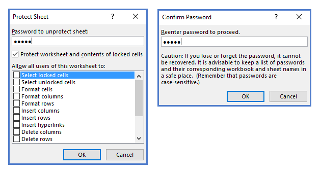 <
<Fig 3: Protect Sheet dialog box - Left: deselect all the items in the "Allow all users of this worksheet to:", then enter a password (90045). Click OK. Right: Confirm Password dialog box - complete the Reenter password to proceed section
2. Code for the Workbook_Open macro enable event
When macros are enabled, either automatically or by the user clicking the Enable Content button, the Workbook_Open macro in code 1 will be executed.
Code 1: Sub
Workbook_Open located in the ThisWorkbook module
Private Sub Workbook_Open()
Dim WS As Worksheet

    For Each WS In Worksheets
        If WS.Name <> "Warning" Then WS.Visible = xlSheetVisible
    Next

    Worksheets("Warning").Visible = xlVeryHidden
    ActiveWindow.DisplayGridlines = True

End Sub
About code 1
- Line 1: The private sub procedure is located in the ThisWorkbook module. The code executes on the Open event of the workbook, but only if Macros are enabled
- Line 2: declare a variable named WS of object type Worksheet
- Lines 4 to 6: Loop through all of the Worksheet objects in the Worksheets collection. Make all of the worksheet visible by setting the Visible property to xlSheetVisible
- Line 8: hide the worksheet named Warning. Visible property set to xlVeryHidden
- Line 9: display the gridlines of all worksheets
3. The code to reset the macro warning
Code 2: Sub
ResetWarning located in an ordinary code module
Private Sub ResetWarning()
Dim WS As Worksheet

    Worksheets("Warning").Visible = True
    ActiveWindow.DisplayGridlines = False
    Range("A1").Select

    For Each WS In Worksheets
        If WS.Name <> "Warning" Then WS.Visible = xlSheetVeryHidden
    Next

End Sub
About code 2
This private macro is used to reset the warning message. It is run either from the VBE, or by manually entering the name in the Excel macro dialog box.
- Lines 18: makes the Warning worksheet tab visible (the reverse of code 1 line 8)
- Lines 19: hide the gridlines of all worksheets (the reverse of code 1 line 9)
- Lines 22 to 24: Loop through all of the Worksheet objects in the Worksheets collection. Make all of the worksheet invisible (veryhidden) by setting the Visible property to xlSheetVeryHidden (the reverse of code 1 lines 4 to 6)
- Download the file: Excel file (xlsm) [57 KB]
- This example was developed in Excel 2016 64 bit with VBA 7.1.
- Revised: Saturday 25th of February 2023 - 10:12 AM, [Australian Eastern Time (AET)]