
Excel worksheet arrays and vectors
This material about arrays and vectors involves three concepts:
- Excel structures able to hold data, most commonly, the array of cells on a worksheet (by reference, name or constant)
- mathematical element wise array operations, and
- matrix based linear algebra array operations
0. Arrays
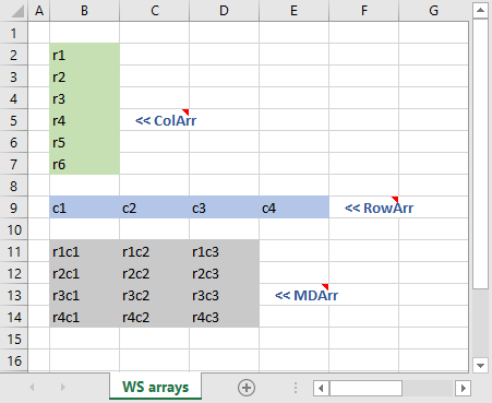
An array can be described as a group of items that can be acted on either individually or collectively. An array's orientation is classified by its dimension (such as column orientation, or row orientation, discussed further in section 1). In Excel the concept is best illustrated by example, see figure 1 (worksheet: WS arrays) where "a group of items" means a contiguous range, In particular, an array can be a:
- Scalar - a single cell
- Column array (column vector) - range
B2:B7shaded green - Row array (row vector) - range
B9:E9shaded blue - Multi dimensional array - range
B11:D14shaded grey
The expressions "scalar", "row vector" and "column vector" are common to the MatLab (matrix laboratory) application software.
1. Arrays - concepts
Dimension
The size of an array is described by the number of rows and number of columns. By convention the dimension is always rows first and columns second, in the spirit of R1C1 reference style, and the ordering of row and column arguments in functions such as INDEX and OFFSET.
Excel uses [mR x nR] during selection resizing operations (m and n are common to MatLab). MatLab uses m x n notation, with m being the number of rows (first dimension) and n being the number of columns (second dimension). Thus [2R x 3C] is a 2 row by 3 column array.
An array is contiguous, meaning rectangular / square, and a worksheet array can be referenced by the top left cell and bottom right cell with the range operator, see B11:DF14 in figure 1. Some functions return an array (eg. the TRANSPOSE and MMULT functions).
Dimensions (from figure 1):
- Scalar: dimension 1 x 1 (not shown in figure)
- Column vector: named
ColArr, dimension 6 x 1, number of elements 6 - Row vector: named
RowArr, dimension 1 x 4, number of elements 4 - MultiDimensional array: a two dimensional array named
MDArr, dimension 4 x 3, number of elements 12
In mathematics, the arrays in figure 1 can presented in the form:
$$\text{ColArr}=\begin{bmatrix} r1 \\ r2 \\ r3 \\ r4 \\ r5 \\ r6 \end{bmatrix}, \qquad \text{RowArr}=\begin{bmatrix} c1 & c2 & c3 & c4 \end{bmatrix} \qquad \text{MDArr}=\begin{bmatrix} r1c1 & r1c2 & r1c3 \\ r2c1 & r2c2 & r2c3 \\ r3c1 & r3c2 & r3c3 \\ r4c1 & r4c2 & r4c3 \end{bmatrix}$$where [ ] represents the array.
Name Manager curly braces "{}"
In Excel there are two representations of arrays:
- the worksheet depiction in figure 1, and
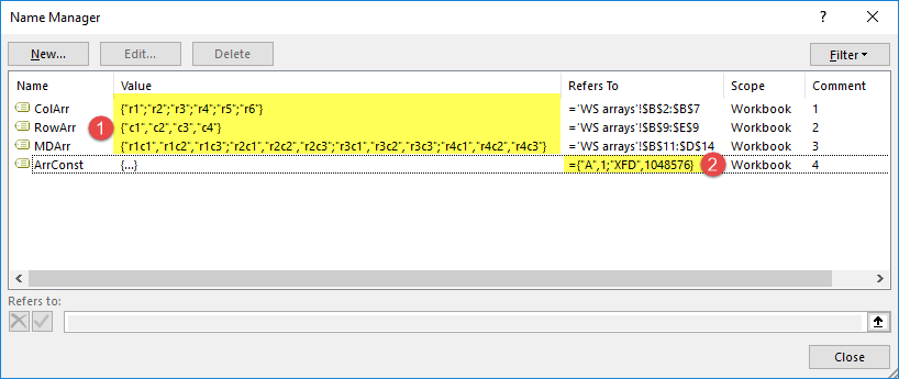
- computer memory depictions such as the Value and Refers To field of the Name Manager (figure 2)
Value field
The three arrays from figure 1 are stored arrays link and are labeled ![]() in figure 2
in figure 2
- Excel arrays use opening "{" and closing "}" curly braces
- Arrays are constructed on a row by row basis
- Individual elements are separated by a comma ","
- End of row is marked by a semi-colon ";" except for the last row
- These formats do not apply to a scalar
In Excel array notation:
- Name:
ColArr; Value:{"r1";"r2";"r3";"r4";"r5";"r6"} - Name:
RowArr; Value:{"c1","c2","c3","c4"} - Name:
MDArr; Value:{"r1c1","r1c2","r1c3";"r2c1","r2c2","r2c3";"r3c1","r3c2","r3c3";"r4c1","r4c2","r4c3"}
"Refers To" field
The array ArrConst, labeled ![]() in figure 2 is a named array constant. It has 2 x 2 dimension and is used in the Named Array Const worksheet in figure 3.
in figure 2 is a named array constant. It has 2 x 2 dimension and is used in the Named Array Const worksheet in figure 3.
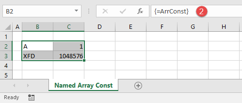
In Excel array notation, the named array constant has:
- Name:
ArrConst; - Value:
{...}curly braces with a horizontal ellipses; - Refers To:
{"A",1;"XFD",1048576}
To enter the array, select a 2 x 2 range, type =ArrConst in the Formula Bar, then press Control + Shift + Enter to complete the formula.
A named array constant
- can contain numbers, text, logical values (TRUE and FALSE) and error values (like #N/A!)
- all text must be in double quotes ""
- cannot contain other arrays, formulas, or functions
- percentages must be decimal or text (0.10 or "10%")
Function Arguments curly braces "{}"
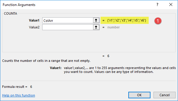
Array values are displayed in the Function Arguments dialog box to the right of the argument name (figure 4). A maximum of 36 characters are shown.
Formula F2 F9 curly braces "{}"
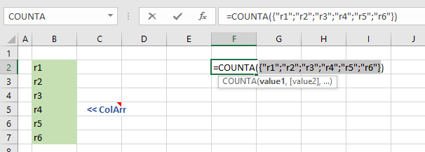
You can check the values in an array (or reference) with the F2 F9 sequence. In figure 5, the cell F2 has the formula =COUNTA(ColArr). To check the values in the array
- switch to Edit mode by pressing F2
- select the reference
ColArrin the Formula Bar - press F9 to debug part of a formula. The result is displayed in the figure
- this technique is limited by the formula maximum of 8,192 characters (2 ^ 13)
2. Arrays - element wise operators
Operations on an array, as described in section 2, requires an array formula which has several distinct features compared to a conventional formula in Excel.
- An array formula is completed by pressing the CONTROL + SHIFT + ENTER key sequence often referred to by the abbreviation CSE formula
- There two distinct types of operations involving arrays
- Element by element, and
- Matrix (based on linear algebra)
- Only element by element is covered in this module
- (Generally) Each array must have the same magnitude and direction. In other words, the name dimension (excluding 1 x 1 scalar arrays)
- You cannot edit or delete part of an array. You must select the current array - use the Ctrl + / shortcut, or Home > Editing > Find & Select > GoTo Special > Current array
Example - Excel Online #1
From the "element wise" worksheet in figure 6. The example uses two row vectors each of dimension (1 x 3). The range names of the arrays and values are: x = [1,2,3], and y = [4,5,6], and they appear in rows 4 and 5 of figure 6
WS1: the element wise worksheet demonstrates:
- Addition
- Subtraction
- Multiplication
- Division
- Scalar addition
- Scalar subtraction
- Scalar multiplication
- Scalar division
- Scalar exponentiation
- Scalar logical
WS2: The U x P >> Sales worksheet demonstrates a small data base of Unit number and Price data, the user is required to:
- Calculate Total Sales using normal cell formulae and the SUM function
- Calculate Total Sales using CSE formulae for sales then SUM
- Calculate Total Sales using CSE formulae in the final cell
- Repeat step 3 using the Excel SUMPRODUCT function
Each vector is 6 x 1.
WS3: The 100 records no IF filter worksheet uses the 100 records data base to demonstrate vector logical CSE formulas. Required:
- Sum product A, B and C for
Salesperson = "Wong" - Sum product A, B and C for
Salesperson = "Wong" AND Month = "September" - Sum product A for
Salesperson = "Wong" AND Product A >= 10 AND Product A <= 30
Each field column uses the label as vector name. For example, the Invoice No field has vector name Invoice_No
The CSE formulas are (in Ready mode):
{=SUM((Salesperson = "Wong") * Prod_C_qty)}{=SUM((Salesperson="Wong") * (Month="September") * Prod_C_qty)}{=SUM((Salesperson="Wong") * (Prod_A_qty >= 10) * (Prod_A_qty <= 30) * Prod_A_qty)}
WS4: The NPV as CSE worksheet uses using the VisiCalc handbook numbers, and the xlf Carrot Washer example.
The technique is a direct interpretation of the NPV equation - $$\begin{equation} NPV=\sum_{t=0}^{n} \frac{C_t}{(1+k)^t} \end{equation}$$ where the initial cash flow at time zero and future cash flows at time \(t\) are denoted \(C_t\) over \(n\) periods. \(k\) is the periodic discount rate.
Using equation 1, the application is:
The VisiCalc example $$ NPV=\frac{-20,000}{(1+0.1)^{0}} + \frac{3,000}{(1+0.1)^{1}} + \frac{7,500}{(1+0.1)^{2}}+ \frac{15,000}{(1+0.1)^{3}}+ \frac{25,000}{(1+0.1)^{4}}+ \frac{30,000}{(1+0.1)^{5}} = \$35,898 $$
The carrot washer example $$ NPV=\frac{-80,000}{(1+0.05)^{0}} + \frac{10,000}{(1+0.05)^{1}} + \frac{20,000}{(1+0.05)^{2}}+ \frac{15,000}{(1+0.05)^{3}}+ \frac{50,000}{(1+0.05)^{4}}+ \frac{20,000}{(1+0.05)^{5}} = \$17,428 $$
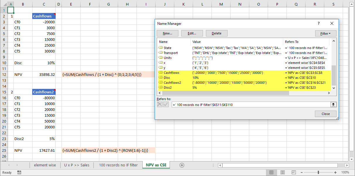
The CSE formulas for the NPV estimates are:
- VisiCalc
=SUM(Cashflows / (1 + Disc) ^ {0;1;2;3;4;5})returns 35,898.32, where{0;1;2;3;4;5}is an array constant (column orientation 6 by 1) - carrot washer
=SUM(Cashflows2 / (1 + Disc2) ^ (ROW(1:6) - 1))returns 17,427.61
- Development platform: Excel 2016 (64 bit) Office 365 ProPlus on Windows 10
- Related material: Add a series of relative offset names to the Name Manager
- O'Connor I, (2015) Convert lower triangle table to full matrix. Includes discussion of array / matrix dimension and element indexing
- O'Connor I, (2017) Excel functions with array arguments. Includes array (CSE) and enter formulas
- O'Connor I, (2015) Vector to array constant. Includes VBA code for text based vector
- Revised: Saturday 25th of February 2023 - 10:12 AM, [Australian Eastern Time (AET)]