
Last known value interpolation of missing data points
There are many techniques available for interpolation of values in time series data (see Alexander (2008) for examples). This module describes the last know value (LKV) interpolation method with application to situations where price-volume data points are missing from a data set.
Missing data could be due to errors in data collection, no trades occurring for a day or sequence of days, or the stock being suspended from trading for a period.
As an example, the company 99 Wuxian Ltd (ASX code NNW.AX) was suspended from official quotation on the ASX from 18 November 2015 until its reinstatement to official quotation on 16 December 2015. The ASX Price-volume chart is in figure 1a, and open-high-low-close chart (described as a daily bar chart by the ASX) is in figure 2b. The last observed price of $0.105 is carried forward over the suspension of trading period, with an associated zero trading volume figure (as marked in the figure). This technique can be described as last known value interpolation. The value is carried forward in real time, without prior knowledge of the resumption of trading value.

Source: http://asx.com.au accessed 9 May 2016
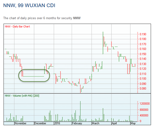
Source: http://asx.com.au accessed 9 May 2016
Depending on the specific reason for the suspension of trading, the last know price is often a good indicator of stock value for investors and other information users, because it is based on information known in the market place.
See the animated graphic in figure 2 for an illustration of the LKV method. In the example, three data points are missing, so the last known value, $12 on 5 May 2016, is carried forward for the period 6 May 2016 to 10 May 2016. Note: LKV interpolation is described as forward-flat interpolation in NumXL time series add-in package.
To implement LKV interpolation in Excel, we need to create some relative reference defined names, and use these in conjunction with the Excel Find and Replace feature.
1. Create the mixed reference and relative reference defined names and Replace with formula
Two LKV techniques are described, each should be obvious from the specifications (points 4 and 5). All specification refer to figure 3, where the Date vector is in column B, and the last data record (11 June 2014) is in row 87. Suppose that the ActiveCell is cell F88 of the worksheet (figure 3), then the specifications of the defined names for the MissingData worksheet are:
- Last know Close. Name: LKClose; RefersTo:
=MissingData!$F87. Equivalent to=MissingData!R[-1]C6in R1C1 reference style - One Above. Name: OneAbove; RefersTo:
=!C87. Equivalent to=!R[-1]Cin R1C1 reference style - Last known Adj Close. Name: KAdjClode; RefersTo:
=MissingData!$H87. Equivalent to=MissingData!R[-1]C8in R1C1 reference style - LKClose Formula
=IF(OR(COLUMN()=6,COLUMN()=8),OneAbove,0). - LKOpen2AdjClose Formula
=IF(COLUMN()<=6,LKClose,IF(COLUMN()=8,LKAdjClose,0)).
2. Replace the #N/A errors with LKV numbers
Using the LKOpen2AdjClose formula from point 5.
- Open the MissingData worksheet, then follow steps 7 to 12 to fill the Open, High, Low, Close with the LKClose values; Volume with 0; and AdjClose with LKAdjClose, plus a yellow highlight to the LKV formulas. The before state is shown in figure 3
- Ensure that the Active Cell in the data region, then press Ctrl + A to select the Current Region
![[Firefox: click for image]](media/xlf-interpolation-lkv-with-na-errors.png)
- Open the Find and Replace dialog box Ctrl + F and select the Replace tab Alt + P. The Find and Replace dialog and sub dialog box are shown in figures 4a to 4d inclusive
- Enter the Find what: and Replace with: values as shown in figure 2a (Paste the Replace With string from the WorkArea location). This specification will relace each #N/A text string with the LKOpen2AdjClose formula
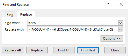

- Remaining in the Replace tab, Click the Options button Alt + T to display the Replace Format dialog box (figure 4c). Then on the Fill tab select Background Color: Yellow (as shown by the pointer)
- Click OK to close the Replace Format dialog box

- Click Replace All Alt A in figure 4d.


When completed, the message box in figure 5 will appear. Click OK. The interpolated data is in figure 6. Manually adjust the first row if necessary.
![[Firefox: click for image]](media/xlf-interpolation-lkv-completed.png)
References
Alexander C, (2008), "Quantitative Methods in Finance", Wiley.
excelatfinance.com, "Add a series of relative offset names to the Name Manager", link Accessed 1 September 2016
- This example was developed in Excel 2016 64 bit.
- Revised: Saturday 25th of February 2023 - 09:37 AM, [Australian Eastern Standard Time (EST)]
LastMod: [2023-02-25AEDT09:37:55+11:00 ]