
x-y scatter plot with correlated random numbers
In this module:
- Random number generator - using volatile functions - with number of observations \(n\) switch
- Dynamic range as a statistical data reference
- Dynamic range as a chart series
- Creating an X Y scatter chart
Random number generator
Pseudo random numbers \(\text{N(0,1) i.i.d.}\) are generated by the Excel RAND function and then passed as the probability argument to the NORM.S.INV function. The correlation structure is incorporated by using the Cholesky decomposition method.
Cholesky decomposition
Generate \(Z_1,Z_2\)
- Generate \(Z_1,Z_2 \sim \text{N(0,1) i.i.d.}\)
- Set \(X=Z_1\) and \(Y=\rho Z_1 + Z_2 \sqrt{1-\rho^2}\), where \(\rho\) is the correlation coefficient
The X Y data worksheet
\(Z_1,Z_2\) are generated on the worksheet named: X Y data. Pseudo random numbers \(\text{N(0,1) i.i.d.}\) are generated with the nested NORM.S.INV(RAND()) formula.
- Cell B3:
=IF(ROW()-2<=NoObs,NORM.S.INV(RAND()),"") - Cell C3:
=IF(ROW()-2<=NoObs,rho*B3+SQRT(1-rho^2)*NORM.S.INV(RAND()),"")whererhoandNoObsare links to the selector and validator panel - Copy
B3:C3and paste to the rangeB4:B5002. NameB3:B5002as X, andC3:C5002as Y
Summary statistics and the X-Y scatter plot
Refer to the X Y Interface worksheet shown in the figure 1 Excel Web App #1.
The selector / validator panel
The correlation selector
- D5: the correlation selector - is set up by Data Validation
- Select Data > Data Tools > Data Validation
- In the Data Validation dialog box - Settings tab
- Set Validation criteria; Allow:
Decimal; Data:between; Minimum:-1; Maximum1 - In the Data Validation dialog box - Input Message tab
- Set Title:
Correlation value; Input message:Enter rho in the range ... -1 <= rho <= +1
The "No of points" validator
- D6: the "No of point"s validator - is set up by Data Validation
- Select Data > Data Tools > Data Validation
- In the Data Validation dialog box - Setting tab
- Set Validation Criteria; Allow:
List; Source:625,1250,2500,5000 - In the Data Validation dialog box - Input Message tab
- Set Title:
Number of observations; Input message:625, 1250, 2500, 5000, ... Select 625 to reduce worksheet recalculation time
The descriptive statistics panel
Note: INDIRECT(D$10) uses the value in cell D10, X, to point to the range named X.
Formulas in the summary statistics section:
- C11:
=MIN(INDIRECT(D$10) - C12:
=MAX(INDIRECT(D$10) - C13:
=AVERAGE(INDIRECT(D$10) - C14:
=VAR.S(INDIRECT(D$10) - C15:
=STDEV.S(INDIRECT(D$10) - C16:
=SKEW(INDIRECT(D$10) - C17:
=KURT(INDIRECT(D$10) - C18:
=COUNT(INDIRECT(D$10) - C19:
=MAX(INDIRECT(D$10)-MIN(INDIRECT(D$10) - C21:
=COVARIANCE.S(X,Y) - C22:
=CORREL(X,Y) - C23:
=COVARIANCE.S(X,Y)/(STDEV.S(X)*STDEV.S(Y))
The X Y scatter plot
- To select the data, type
XV,YVin the Name Box. If you are using the Web App file, you will need to Unhide theX Y dataworksheet before you select the data. Create the chart on that worksheet, then move it to theX Y interfaceworksheet - Insert the chart - follow the ribbon sequence: Insert > Charts > Charts Dialog Launcher > All Charts tab > X Y (Scatter) > Scatter. Click OK to display the chart shown in figure 2
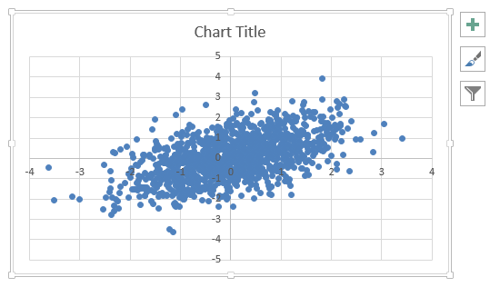
Fig 2: X Y Scatter plot - with Number of points set to 1,250 - Using the Insert > Chart sequence does not retain the reference to the dynamic range names, instead a static name is applied (see figure 4). When a vector length shorter than the static range is selected, the X Y chart collapses as shown in figure 3. The x axis (the Horizontal (Value) Axis) displays the observation numbers, with the observation 626 onwards displaying as blank (the static vector being 1,250 data points in length)
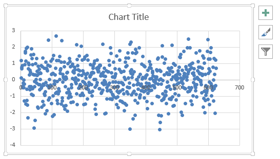
Fig 3: X Y Scatter plot - with Number of points set to 625. The scatter plot has collapsed because the Series references are static - To display the Edit Series dialog box, use the ribbon sequence Design > Data > Select Data to display the Select Data Source dialog box, then, in Legend Entries (Series) select
Series1, then click Edit. The Edit Series dialog box will now be displayed - figure 4 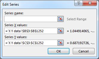
Fig 4: X Y Scatter - Edit Series dialog box - showing that Series Values are static - hard coded references - In step 1, the dynamic ranges
XYandYVwere selected, but these were overwritten by Series X values:='X Y data!$B$3:$B$1252and Series Y values:='X Y data!$C$3:$C$1252as shown in the Edit Series dialog box in figure 4. The series reference need to be replaced with links to the dynamic vectors - Link the chart series to the dynamic range - by editing the series values. Set Series X values:
='xlf-x-y-scatter.xlsx'!XV, and Series Y values:='xlf-x-y-scatter.xlsx'!YV - Format the X Y chart - from the Chart Tools tab, select Format > Current Selection > Chart Elements box then the Chart Area element.
- From the same ribbon tab, select Size, and set
Height: 12.5 cm, andWidth: 12.5 cm - A two vector X Y plot has only one series, and the Series name value in figure 4 was left blank, thus the default name is Series1. Select Series1 from the Chart Element box
- Click Format Selection to display the Format Data Series task pane. This is the Office 2013 implementation of an Office 2010 dialog box. An example is shown in figure 5

Fig 5: Excel 2013 task pane - showing Format Data Series options - Select Marker > Marker Options, then Built-in, and set Size:
2 - Select Series Options > Horizontal (Value) Axis. This will display the Format Axis task pane
- Select Axis Options (the three column icon), then set Bounds; Minimum:
-4.0, and Maximum:4.0. Vertical axis crosses; Axis value:0.0 - Repeat step 10 for the Vertical (value) Axis. Select the axis from the Axis Options > Elements List box - figure 6
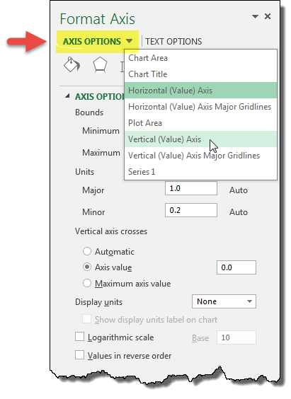
Fig 6: Format Axis task pane - showing Axis Options elements list - Add a trendline - to display the Format Trendline task pane.
- Select the Fill & Line tab, then set Line:
Solid; Color:Standard Colors, Red; Width:1.5 pt; Dash type:Solid; then Close the task pane. - Hide the chart title - Chart Tools > Design > Add Chart Elements > Chart Title > None
- Cut and paste the chart to the
X Y interfaceworksheet - The completed chart appears in figure 7
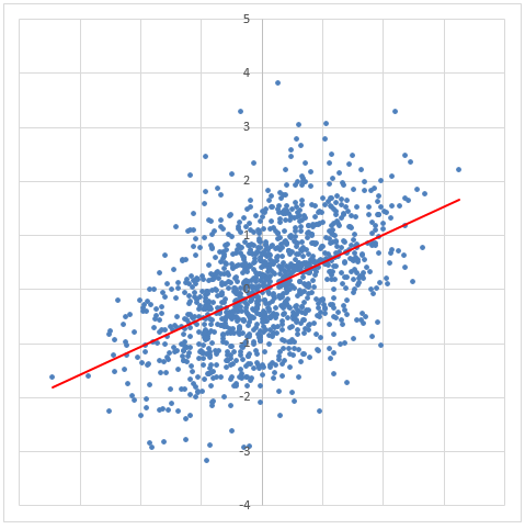
Fig 7: X Y scatter - completed. Includes gridlines. Selector / validator options set to correlation 0.5 and 1250 points
Selected Excel functions used in this module and associated statistical functions.
| Excel functions | Description |
|---|---|
| NORM.S.INV(probability) [2010] | Returns the inverse of the standard normal cumulative distribution \(\text{N(0,1) i.i.d.}\). |
| RAND() | Returns an evenly distributed random number \(0 \le x \lt 1\). The rand function takes no arguments |
| ROW([reference]) | Returns the row number of a reference |
| SQRT(number) | Returns the positive square root of a number \(\sqrt{x}; \quad x^{0.5} \) |
- This example was developed in Excel 2013 Pro 64 bit.
- Published: 2 September 2015
- Revised: Saturday 25th of February 2023 - 10:13 AM, [Australian Eastern Standard Time (EST)]