
portfolio analysis - Excel
A portfolio can be viewed as a combination of assets held by an investor.
For each asset held, such as company stocks, the logarithmic or continuously compounded rate of return \(r\) at time \(t\) is given by $$ r_t = \log \left(\frac {P_t} {P_{t-1}} \right) $$ where \(P_t\) is the stock price at time \(t\), and \(P_{t-1}\) is the price in the prior period.
The volatility of stock returns, over time \(N\) is often estimated by the sample variance \(\sigma^2\) $$ \sigma^2 = \sum \limits_{t=1}^N {\frac {(r_t - \bar r)^2} {n - 1}} $$ where \(r_t\) is the return realized in period \(t\), \(\bar r\) is the sample mean, and \(N\) is the number of periods. As the variance of returns is in units of percent squared, we take the square root of the variance to determine the standard deviation $$ \sigma = \sqrt { \sum \limits_{t=1}^N {\frac {(r_t - \bar r)^2} {n - 1}}}$$
Suppose an investor has a four stock portfolio comprising of shares on the Australian stock market (AGK, CSL, SPN, and SKT) as listed in figure 1.
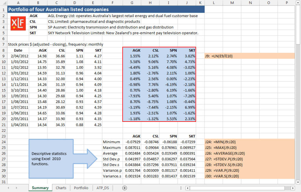
The companies with stock codes AGK, CSL, SPN, and SKT are:
- AGK: AGL Energy Ltd - operates Australia's largest retail energy and dual fuel customer base
- CSL: CSL Limited - pharmaceutical and diagnostic products
- SPN: SP Ausnet - electricity transmission and distribution, and gas distribution
- SKT: SKY Network Television Limited - New Zealand's preeminent pay television operator
These stock were chosen because they have positive returns during the sample period.
1. Descriptive statistics
Price data for the four stock is obtained from Yahoo Finance and is filtered for monthly price observations. In figure 1, Column A of the Summary worksheet shows the date for the first trading day of the month. Closing prices for the four stock are in the range B9:J21. The corresponding continuously compounded return series, using the Excel LN function, is calculated in the range G9:J20. Summary statistics from Excel functions: MIN, MAX, AVERAGE, STDEV.P, STDEV.S, VAR.P, and VAR.S are in rows 24 to 29.
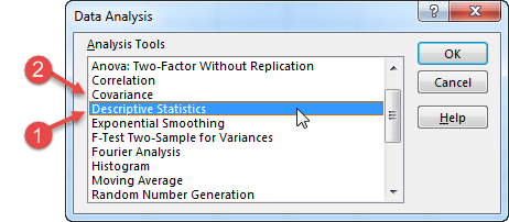
Descriptive statistics can also be estimated by using the Descriptive Statistics item, from the Data Analysis dialog box (figure 2, item 1), as shown in figure 3.
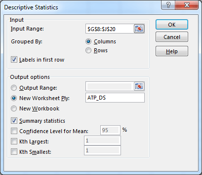
The output for the Descriptive Statistics, with setting from figure 3, is shown in the New Worksheet ply, ATP_DS in figure 4.
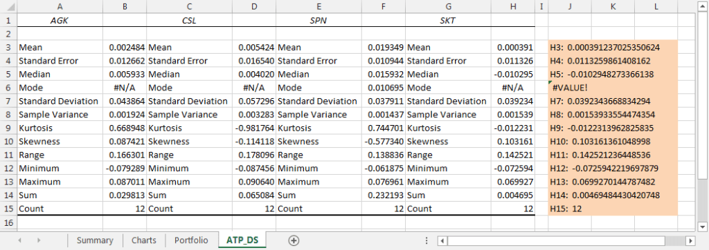
Rows 7 and 8 of the worksheet in figure 4 have values for the sample standard deviation (row 7) and sample variance (row 8). We will see later, that the Data Analysis > Covariance item returns population values, not sample values.
Limitations of the ATP Descriptive Statistics
- The table of values is static. It is not linked to the source data, and the Descriptive Statistics dialog box must be reactivated to update the values
- Each row vector in the table has alternate labels and values. This means it is not conducive to using the values as a vector in other calculations such as weighted average portfolio return
When assets are held as part of a portfolio, another important consideration is the amount of co-movement between the returns of portfolio components.
2. Covariance
The degree of co-movement can be measured by the covariance statistic, and is calculated on a pair-wise basis. The formula for the sample covariance \(\sigma_{i,j}\) for the return vectors of stock \(i\) and stock \(j\) is $$ \sigma_{i,j} = \sum \limits_{t=1}^N {\frac {(r_{i,t} - \bar {r_i})(r_{j,t} - \bar {r_j})} {n - 1}} $$
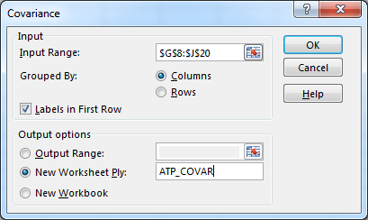
There are a number of ways the estimation can be operationalised and some techniques are described in this section. Methods include the Analysis Toolpak - Covariance item (figure 2, item 2), and Excel function listed in the following table.
| Excel covariance functions | Description |
|---|---|
| COVARIANCE.P(array1, array2) | Returns the population covariance, the average of the product of paired deviations \(\sigma_{i,j} = \sum \limits_{t=1}^N {\frac {(r_{i,t} - \bar {r_i})(r_{j,t} - \bar {r_j})} {n}}\) |
| COVARIANCE.S(array1, array2) | Returns the sample covariance, the average of the product deviations for each point pair in two data sets \(\sigma_{i,j} = \sum \limits_{t=1}^N {\frac {(r_{i,t} - \bar {r_i})(r_{j,t} - \bar {r_j})} {n - 1}}\) |
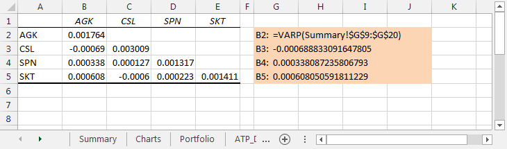
The worksheet in figure 6 shows output for the Analysis Toolpak (ATP) covariance item in rows 2 to 5. The covariance table from the ATP is lower triangular, meaning it only returns the main diagonal elements, and the lower left elements. By definition, the covariance of a vector with itself, is the variance of the vector. Thus, the value in cell B2 in figure 6, \(\sigma_{AGK,AGK} = 0.001764\) is the same value as the population variance returned by the Excel VARIANCE.P function shown in figure 1 cell G30. To convert the lower triangular table to a full matrix see - lower triangular table to full matrix
In figure 7, rows 41 to 44, use the COVARIANCE.P function with Excel range names for each of the return vectors. This is repeated with the COVARIANCE.S function in rows 48 to 51.

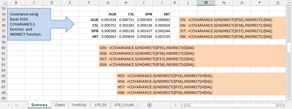
Construction of the individual cell formulas can be simplified by using range names with the INDIRECT function.
To do this:
- Copy and paste the stock code vector to the range as column headings
- Using Paste Special > Transpose, paste the transposed stock codes vector to form row headings
- Enter the formula
=COVARIANCE.P(INDIRECT(F$55),INDIRECT($G54))at G55
The returned values, and cell formulas are shown in figure 8.
Download the file for this module from the figure 8 Excel Web App #1 link
Links to related information
- Continuously compounded rate of return: Rate of return
- Convert a lower triangular table to full matrix: Lower triangular table
- This example was developed in Excel 2013 Pro 64 bit.
- Published: 7 September 2015
- Revised: Saturday 25th of February 2023 - 10:13 AM, [Australian Eastern Standard Time (EST)]