Version 2

A price-volume chart shows two series in the one Excel chart, and is often referred to as a combination or combo chart. Price is the primary \(y\) axis, Volume is the secondary \(y\) axis, and the Date vector in on the horizontal \(x\) axis.

Two particular features of the price-volume time series dates are addressed in this module:

1. The Date vector of the source data is in descending order. It is customary, however, that the chart date axis be in ascending order, and
2. The Excel chart date axis automatically includes all calendar days. In practice, however, the axis should include actual trading days only

Example: this module is based on one month of stock price volume data for the company Bank of Queensland Ltd – Australian stock exchange code – BOQ.AX. The data source for the BOQ.AX price volume series for the month of July 2014, is Yahoo Finance.

The data has seven fields, labeled \(Date, … , Adj \ Close\). You can download the sample file from the Excel Web App download link in figure 1.

A log return vector, labeled Returns has been added to column H in the Data BOQ.AX worksheet. The log return \(r_t=log(P_t/P_{t-1})\) is the log transform of the adjusted closing price series using the Excel LN function.

Important: Normally the issues described in points 1 and 2 above can be solved by converting the \(x\) axis date vector to text, and displaying the series in reverse order. This works in the case of a single chart series, but fails in the case of a combination chart, as only one of the series reverses to match the dates. The second series does not reverse its order to match the dates.

The obvious solution is to sort the data on the date column in ascending order, or construct a specific range with dates in ascending order for the chart series. The latter method is adopted here and described in item 2 below.

Create a price volume chart in Excel 2013

1. Data series (noncontiguous) sorted on Date vector: in the original data series on the Data BOQ.AX worksheet, the Date range, A2:H25 is not adjacent to the Volume / Price range. This means that the Date, Volume and Price series are noncontiguous and cannot be selected as a block.

1. Select the noncontiguous series:
   • Using the mouse – press Ctrl + click and drag to select the Date vector (column A), and then the Volume / Price array (columns F and G), or
   • Enter the noncontiguous range in a cell of your work area, $A$2:$A$24,$F$2:$G$24, then copy and paste to the Name Box, or the F5 dialog. This method is useful when the series range is large, and may save retyping the address.

2. Data series (contiguous) workarea range: Create a linked reverse order target, PriceVolumeChart as shown in figure 2. This allows the structure of the source data on the Data BOQ.AX worksheet to remain unaltered, ie. in descending order.
   • Let the Date vector in column A of the Data BOQ.AX worksheet have the name DateV.
   • Use the Excel INDEX function to link the DateV source to the reverse order target vector revDateV

1. Syntax: INDEX(array,row_num,column_num) where INDEX returns the value in the cell at the intersection of row_num and column_num

   • The equation to link the reversed target is =INDEX(DateV,ROWS(DateV)-(ROW()-ROW(revDref)-2),1)
   • This is then wrapped in an IFERROR function =IFERROR(INDEX(DateV,ROWS(DateV)-(ROW()-ROW(revDref)-2),1),"") to handle the case where the revDateV target is longer than the DateV source. Create a revDateData range with enough rows to accommodate the maximum number of observations in the analysis window. In other words, the maximum length of the DateV range plus 1.

1. 

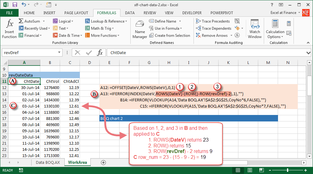
   Fig 2: The revDateData reverse order date vector, revDateV The INDEX function row_num argument is anchored to cell A11, marked ? in the WorkArea worksheet:

   • In figure 2, cell A11, marked ? has the name revDref, and the item ? displays the formula in cell A13. Attaching the anchor to a label rather than a formula avoids the first row of the formulas for ChtVal and ChtAdCl being linked to a name reference with absolute addressing
   • Items ? ? and ? are the components of the row_num parameter to the INDEX function
   • The revDateV vector starts in row 13, ie. cell A13. The formula is cell A12, linking to the 30 June 2014 allows for inclusion of a returns vector at a later stage.
   • How it Works: a discussion of the equation in cell A15, denoted ? in figure 2. Looking at the DateV vector in figure 1, the date 3 July 2014 is element number 21 with base 0. This is also the 3rd last element in the source (figure 1), and it is the 3rd element in the revDref target (figure 2).
   • In ?, item ? returns the number of rows in the DateV vector. The value 23.
   • Item ? returns the row number of the formula. The value 15 which is easily verified.
   • Item 3 returns the row number of the revDref cell. The value 11.
   • Thus, the value of items ? ? and ?, is \(23-(15-9-2)=19\) where the 2 is an adjustment to align the relevant bases.
   • Assign dynamic range names to the three vectors in figure 2
     • Name revDateV; Refers to =OFFSET(revDref,2,0,COUNT(DateV)). This vector is the anchor (reference) for the ChtVol and ChtAdCl.
     • Name ChtVol; Refers to =OFFSET(revDateV,0,1). One (1) column to the right of revDateV.
     • Name ChtAdCl; Refers to =OFFSET(revDateV,0,2). Two (2) columns to the right of revDateV.
   • Select the contiguous revDateV data range for July 2014: select the range WorkArea!A13:C35 in figure 2. Selecting columns A to C is important, but the number of rows selected is simply a temporary place holder to be replaced by the dynamic range names.

3. Insert (the chart): On the ribbon, select the Insert > Charts > See all charts sequence to display the Insert Chart dialog. The See all charts item is in the bottom right corner of the ribbon Charts group.
4. Then, on the Insert Chart dialog, select the All Charts tab, then select the Combo item at the bottom of the left column as shown in figure 3. Then on the upper right, select the Clustered Column – Line item. Click the OK button.
5. 

   Fig 3: On the All charts tab, select Combo in the left column, then the Clustered Column - Line item

4. Chart type and axis for series: Currently Volume is Series1 (blue), and Price is Series2 (orange) as identified by the colours. Place the Volume axis on the left, by ticking the Secondary Axis box at the right of Series Name: Series1, Chart Type: Clustered Column in figure 2. This also activates the Custom Combination item, the forth image to the right of Clustered Column-Line. Click OK. The resultant chart is shown in figure 3.
5. 

   Fig 3: Draft version of the Price Volume chart – the format needs improvement

5. Assign the dynamic range names to the chart series by following the steps in the xlfImageGallery. Click an image to view the details.
   • Step 1: Right click the chart background and select the Select Data item, then select Series1, and click Edit.
   • Follow the remaining steps 2 to 5 inclusive.

   

   Step 1: In the Select Data Source dialogue – Ⓐ Select the series, then Ⓑ click Edit.

   

   Step 2: Use your mouse to select the range coordinates, then press Delete to clear the selected coordinates

   

   Step 3: Press F3 to display the Paste Names dialogue. Select the ChtVol Name and then click OK

   
   

   

   Step 4: The Series values now refers to the ChtVol range on the WorkArea worksheet. Click OK

   

   Step 5: If you repeat step 1 to Edit the series you will see that the Workbook name, and Range name are now the Series 1 reference

   
   
   • Step 5: The dynamic range for the ChtVol series is 'xlf-chart-data-2.xlsx'!ChtVol. Note: The address could have been typed directly in step 2. The single quotes around the workbook name are required because the name includes non alphanumeric minus characters.
   • Repeat the five steps to apply the ChtAdCl name and the revDateV name.

6. To eliminate the non trading day gaps in the date vector, select the Horizontal (Category) axis, then click the Format Axis item. See figure 4 for details.
7. 

   Fig 4: Format axis Horizontal (category) axis – axis type = text, with a 5 unit interval

Format the chart

7. Remove the Chart Title and Series labels: Ensure that the Chart is selected – its name will appear in the Excel Name Box. On the ribbon select the sequence Chart tools > Design > Chart Layouts > Add Chart Element. To reduce chart clutter, remove the Chart Title by selecting Chart Title > None. Remove the Series labels by selecting Legend > None.
8. Format the Primary and Secondary axes. This entry was posted on 15 Nov 2014 by xlf ian.